Statistical Rethinking 2026, A04

My solution to exercise A04 from Richard McElreath’s Statistical Rethinking course.

Link to full course on GitHub
Link to online lecture

TipExercise

Using the Howell1 dataset, consider only the people younger than 13 years old. In this sample, estimate the causal effect of each month of growth on weight. Be sure to perform a prior predictive simulation to check and justify your priors. Also try to perform a validation of your model on synthetic data.

Prepare data

First, let’s load the package and data. Then, we’ll keep only those younger than 13 and multiply age by 12 to get age in months.

library(rethinking)
data(Howell1)
d <- Howell1

d <- d[d$age < 13, ]
d$age_months <- d$age * 12

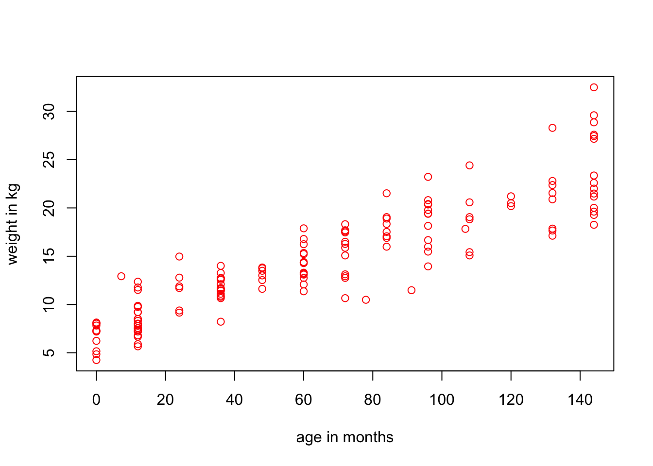
Now let’s make a simple plot and visualize the weight of the children by age.

plot(
  weight ~ age_months,
  data = d,
  col = "red",
  xlab = "age in months",
  ylab = "weight in kg"
)

Statistical model

We will rely on a linear regression that predicts average weight (kg) depending on age (months).

This is the model:

\[ \text{weight} \sim \mathcal{N}(\mu, \sigma) \] \[ \mu = \alpha + \beta (\text{age}_i - \overline{age}) \]

Now we can set some priors. We’ll start with very standard / boring priors.

\[ \alpha \sim \mathcal{N}(0, 10) \] \[ \beta \sim \text{Uniform}(0, 1) \]

\[ \sigma \sim \text{Uniform}(0, 5) \]

Prior predictive simulation

Let’s plot some lines from our model before letting it look at the data:

n <- 1000
a <- rnorm(n, 0, 10)
b <- runif(n, 0, 1)

plot(
  NULL,
  xlim = c(0, 180),
  ylim = c(0, 40),
  xlab = "age (months)",
  ylab = "weight (kg)"
)
mtext("a ~ dnorm(0,10), b ~ dunif(0,1)")

for (j in 1:100) {
  abline(a = a[j], b = b[j], lwd = 2, col = 2)
}

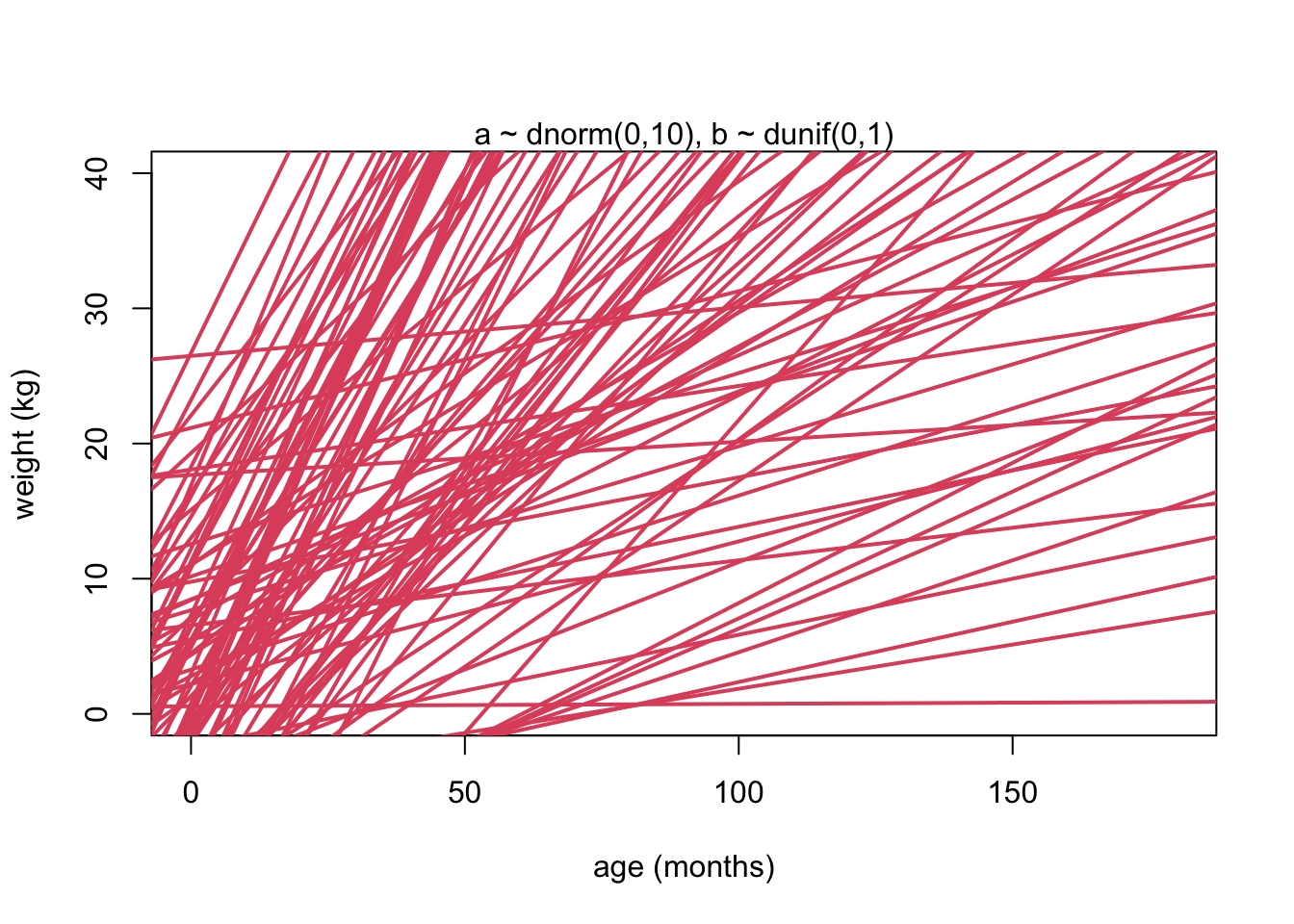
This is not perfect, but as McElreath said in his lecture: “There are no correct priors, only scientifically justifiable priors”.

Simulation-based validation

Let’s now generate synthetic data from our model and see if it makes any sense.

Simulate data

We need a function to generate age and weight data of hypothetical people.

sim_age_weight <- function(N, b, a) {
  age_months <- runif(N, 0, 13) * 12
  weight <- a + b * age_months + rnorm(N, 0, 2)
  data.frame(age_months, weight)
}

dat <- sim_age_weight(1000, 0.3, 0)

head(dat)

  age_months   weight
1   93.31731 28.39965
2   49.39130 14.14093
3   77.59504 23.36225
4   74.09594 19.16934
5   48.36422 13.70640
6  146.98862 42.88791

Let’s have a look:

plot(
  weight ~ age_months,
  data = dat,
  col = "red",
  xlab = "age (months)",
  ylab = "weight (kg)"
)

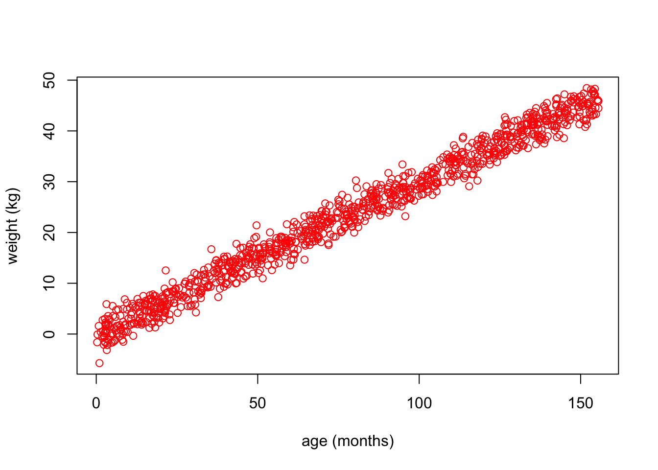
Okay, a bit too linear maybe, but that’s fine. Nothing impossible!

Fit model

Let’s fit our model to this synthetic data:

age_mean <- mean(dat$age_months)

model_synth <- quap(
  alist(
    weight ~ dnorm(mu, sigma),
    mu <- a + b * (age_months - age_mean),
    a ~ dnorm(0, 10),
    b ~ dunif(0, 1),
    sigma ~ dunif(0, 5)
  ),
  data = dat
)

p <- precis(model_synth)
p

            mean          sd      5.5%      94.5%
a     23.2742276 0.063390000 23.172918 23.3755371
b      0.2994172 0.001394192  0.297189  0.3016453
sigma  2.0046080 0.044832984  1.932956  2.0762597

Okay so we’ve successfully recovered b = 0.3 from our data simulation, but what about a? We’ve set a = 0 in the simulation, but now it’s 23.27?
Fortunately that’s not a bug! sim_age_weight() defines a as weight at age = 0, but our fitted model centers on age_mean, so the fitted a is weight at the mean age instead. b doesn’t care about centering, so it comes back correctly.

Visualize

Let’s plot the simulated data (red) & the posterior mean regression line (black):

post_rand <- extract.samples(model_synth, n = 20)
post_full <- extract.samples(model_synth)
a_map <- mean(post_full$a)
b_map <- mean(post_full$b)

plot(
  weight ~ age_months,
  data = dat,
  col = "red",
  xlab = "age (months)",
  ylab = "weight (kg)"
)
mtext("N = 157")

for (i in 1:20) {
  curve(
    post_rand$a[i] + post_rand$b[i] * (x - age_mean),
    col = col.alpha("grey", 0.4),
    add = TRUE
  )
}

curve(a_map + b_map * (x - age_mean), add = TRUE, col = "black", lwd = 2)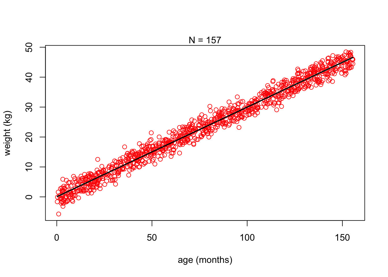

Great!! :)

Fit the model to the real data

For the regression model, we also need the mean age:

age_mean <- mean(d$age_months)

Fit model

Let’s try and fit that model using the rethinking package!

mA4 <- quap(
  alist(
    weight ~ dnorm(mu, sigma),
    mu <- a + b * (age_months - age_mean),
    a ~ dnorm(0, 10),
    b ~ dunif(0, 1),
    sigma ~ dunif(0, 5)
  ),
  data = d
)

precis(mA4)

            mean          sd       5.5%      94.5%
a     14.6869185 0.208855603 14.3531269 15.0207101
b      0.1118122 0.004567271  0.1045128  0.1191116
sigma  2.5241462 0.147715345  2.2880685  2.7602238

Visualize

Okay, now let’s look at the data and the line at the posterior mean plotted (black) and 20 samples from the posterior (grey):

post_rand <- extract.samples(mA4, n = 20)
post_full <- extract.samples(mA4)
a_map <- mean(post_full$a)
b_map <- mean(post_full$b)

plot(
  weight ~ age_months,
  data = d,
  col = "red",
  xlab = "age in months",
  ylab = "weight in kg"
)
mtext("N = 157")

for (i in 1:20) {
  curve(
    post_rand$a[i] + post_rand$b[i] * (x - age_mean),
    col = col.alpha("grey", 0.4),
    add = TRUE
  )
}

curve(a_map + b_map * (x - age_mean), add = TRUE, col = "black", lwd = 2)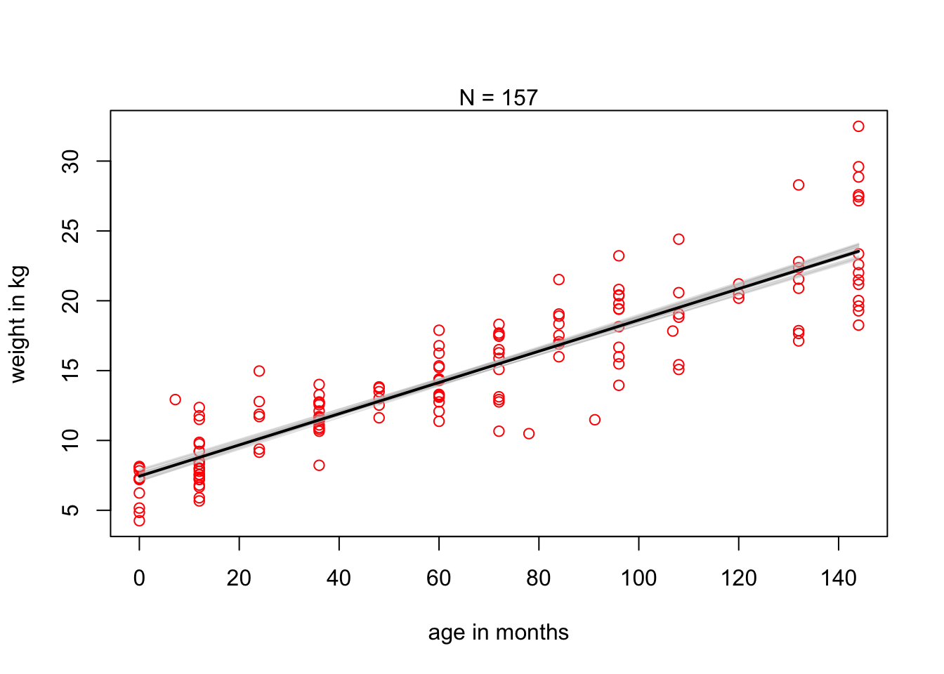

If we had less data (n = 20), then the uncertainty would be larger:

d_small <- d[1:20, ]
mean_age_small <- mean(d_small$age_months)

mA4_small <- quap(
  alist(
    weight ~ dnorm(mu, sigma),
    mu <- a + b * (age_months - mean_age_small),
    a ~ dnorm(0, 10),
    b ~ dunif(0, 1),
    sigma ~ dunif(0, 5)
  ),
  data = d_small
)

post_rand <- extract.samples(mA4_small, n = 20)
post_full <- extract.samples(mA4_small)
a_map <- mean(post_full$a)
b_map <- mean(post_full$b)

plot(
  weight ~ age_months,
  data = d_small,
  col = "red",
  xlab = "age in months",
  ylab = "weight in kg"
)

for (i in 1:20) {
  curve(
    post_rand$a[i] + post_rand$b[i] * (x - mean_age_small),
    col = col.alpha("grey", 0.4),
    add = TRUE
  )
}

curve(a_map + b_map * (x - mean_age_small), col = "black", lwd = 2, add = T)

mtext("N = 20")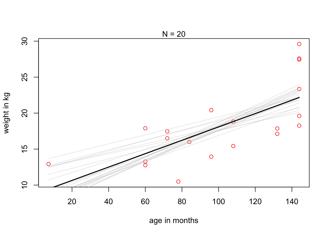

So, what’s the answer? For children under 13, each extra month of age adds about 0.11 kg of weight on average. The simulation-based validation showed that the model recovers the true slope, and the n = 20 version shows what happens with less data: same trend, way more uncertainty. A straight line is of course a simplification — growth isn’t linear from birth to age 13, but it does the job here.